Traveling Surveyor: Contributions of Mahalanobis to Analytics - 2

Bengal
This post is the second in a series of blogs based on the work done by P. C. Mahalanobis in the area of statistics, analytics, and operations research between 1930-1960. We move north-east from the location of our prior post on storm-flood forecasting (Orissa) to Bengal: a land of science, wisdom, and dharma that gave to the world a Vivekananda whose thoughts deeply affected Gandhi's contribution to India's freedom struggle, who in turn shaped the work of Martin Luther King, Jr., and Nelson Mandela, and thus the civil liberties of a significant population of the world.

Much of discussion here is gleaned from ISI archives, websites, and various papers from Sankhya, ISI's flagship journal. Those interested in a more detailed and accurate analysis of this work are referred directly to ISI's journal material.

Jute
Bengal (including Bangladesh, formerly East Bengal) produces much of the world's jute. India is the largest producer and consumer of Jute today, followed by Bangladesh. Jute is an incredibly useful crop and has been a significant contributor to Bengal's revenue for a long time.  Here are some contemporary pictures of standing Jute crop in Bengal.

(pics source: informedfarmers.com)

Why this work is important
Prior to 1947, when India was still occupied by the British Raj (there's a very relevant reason for bringing this up, but we'll get to that later), forecasting the supply of this valuable and lucrative crop in Bengal was largely a product of bad guesswork. Like most other sectors in India, the agricultural sector too is highly decentralized, which means a myriad of tiny farms growing jute and other crops, all of which had to be surveyed if one wanted to get an exact, enumerated production number. Mahalanobis came up with an alternative in the 1930-40s using methods derived from statistics and a field that is now termed 'Operations Research': a scarce-resource optimized method for accurate crop forecasting. Today, the Government of India employs sophisticated remote sensing including a Satellite Survey System to improve crop forecasts, but the methods developed then are still relevant and valuable. The seminal work of Mahalanobis in developing an optimal sample-based survey is also interesting to read from a practitioner's perspective. The combination of ideas employed in the work done in the 1930s include data analysis, statistical modeling, pilot study, scarce resource allocation, and mathematical optimization, and ranks among the great achievements in the practice of Operations Research and Analytics.

A map of undivided Bengal, circa 1850 C. E. (source: http://jrahman.files.wordpress.com)

Motivation
Jute and cotton were two of the most important exports out of India after the manufacturing sectors was crippled by the British Raj - 24% of the total revenue between 1927-37 was from Jute. Estimating the total Jute produce in Bengal up until the 1940s was largely a product of guesswork and ad-hoc estimates provided by the administrative chain of the British Raj produced wildly varying numbers. Like other parts of India, cultivation in Bengal was decentralized and spread over nearly 100 Million small farms, which were on average less than half-an-acre in area, spread over more than 60, 000 sq. miles. Jute was grown in a subset of these farms. Furthermore, the cultivation lifecycle of Jute is very short - about two months from planting to harvesting. Consequently, even if the administration was willing to cough up the expenses for an enumeration survey, covering all these farms within 8-9 weeks would be extremely expensive, if not impossible. Add to the fact, that many plots (30%) that cultivated Jute also cultivated other crops in parallel. Thus, while in theory, we can expect a total enumeration to give us near-zero error, in practice, allotting multi-crop areas to Jute and other Human-induced errors would introduce noise. In fact, the report states that the biggest negative associated with an enumerative survey was not the prohibitive cost but its unreliability, and this motivated Mahalanobis to develop and implement an alternative approach that accomplished the task at a fraction of the cost and time, and at a higher level of accuracy using random sampling.

Random Sampling
The nearly 100M jute farms were spread over Bengal in a non-homogeneous manner. Some areas were densely cultivated, some sparsely. The approach was to partition the total area into zones, i = 1, ..., n (area A_i) whose area was internally homogeneous (kinda like the way finite element analysis is used in structural engineering). Within each zone, a number of areas or grids were selected and sampled at random. If a sufficient number of such grids were sampled, the average proportion of area under Jute within a zone (J_i) can be obtained, which allows us to predict the total area under Jute  = sum(i) A_i * J_i.

Decision variables
1. The partition of the total area into approximately homogeneous zones
2. The number of random samples within a zone
3. The area of a sample

For simplicity, we assume that the first decision of partitioning the area within Bengal is an external input and thus our focus is on optimizing the remaining two decisions.

Constraints
1. The cost of the whole operation depends on the second and third set of decision variables.  For a given budget, if the area of an individual sample is large, then the number of samples has to be reduced, and thus the samples would be more spread out and further away from each other.

2. The achievable precision (variance) varies similarly. If the sample area is large, the per-sample variance is smaller, but cost considerations limited the number of such large-samples, and this can hurt the overall variance accumulated across the zone. On the other hand, a smaller area in tandem with a larger number of such small-samples affects precision in an opposite manner.

Nonlinear Optimization Problem
Given either cost or precision as a hard constraint, select the sampling area and the number of random samples to maximize precision, or minimize cost.

Mahalanobis' approach attempts to model the change in variance and cost as continuous functions of the two decision variable sets. Once these functions are at hand, a local optimum is obtained using a derivative based Lagrange-multiplier method. Mahalanobis used this approach to tabulate the achievable precision for a range of cost levels.

An exploratory, small-scale (pilot) survey was initially conducted at a small expense as a proof-of-concept and proof-of-technology validation of the methodology prior to embarking on a full-scale project. This type of an approach is now widely adopted in many business analytics projects.

The effect of the decision variables on variance can be calculated relying on theoretical methods. However, human-induced errors were also common, and Mahalanobis used the idea of interpenetrating half-sample pairs, where two groups independently arrived at Jute area estimates for a given location.  There are many important details here that are left out for brevity. The cost calculation is detailed and empirical and depends on the nature of the survey, and among things, include:
a. cost of staying and surveying at a given site - this depends on the size of the sampled area and time spent
b. cost of traveling from sample to sample - this depends on the distances between the chosen samples and the sequence of visiting.

Again, we have left out a humongous amount of cost calculations that were done. Reading the reports that came out of this work, one is amazed by the time and effort devoted to meticulously tabulating the various costs that go beyond 'ball-park' estimates, to produce an accurate cost function. For example cost calculation (b) depends on the solution to the corresponding traveling salesman problem.

The TSP
One of the many reports that came out of this this project notes:

(source: Sankhya journal, 1940)

This cost calculation is reviewed by Applegate, Bixby, et al. in their book on TSP and in Bill Cook's 'In Pursuit of the Traveling Salesman'.  A literature review of this TSP in these books mention that researchers later showed that the expected length of the optimal tour was approximately between (0.707, 1.27) times the square root of the number of samples visited in a unit square, so Mahalanobis' 1930s estimate was a remarkably good choice.

Results and Business Impact
The cost- and precision-controlled random sampling approach proved to be revolutionary. It achieved greater precision at a fraction of the cost.  Specifically, the margin of error was +/- 2%, and the cost was 1/15 of an enumeration census that was performed the same year and found to be less accurate compared to the random sampling approach. Thus the benefit and return-on-investment of this analytical approach was successfully demonstrated in practice, which received widespread recognition and was later embraced by the Government of independent India for many nationwide surveys.

Prelude to Part-3: The Bengal Holocaust
Within a couple years of the successful demonstration and publication of this work, Mahalanobis' Bengal lost between 2-6 million people due to starvation and disease between 1942-1945, triggered in part possibly by a failure of rice crop. The British Raj, locked in an grim Atlantic battle during WW2, may have suppressed reports and figures. It appears that most of the world, and even a vast majority of Indians, to this day, remain unaware of the reality behind this event.  How to obtain a reasonable estimate of casualties due to this disaster? Who was responsible and how? A recent book has brought this controversy into the open, and it appears that Mahalanobis (and his statistical sampling method) may have played a critical part in solving this puzzle.

To be continued.

Storm Chaser: Contributions of Mahalanobis to Analytics - 1

Introduction
The recent history of the practice of Analytics and Operations Research in India appears to begin with P. C. Mahalanobis; or at the very least, he is central to this history during the 1930s-1960s time frame.

(source: www.isical.ac.in)

Aside from the well-known Indian Statistical Institute in Kolkata and the distance measure named after him, his legacy includes a rich body of practical analytics work. Examples includes the design of a cost-effective and accurate random sampling method to determine the jute crop output in Bengal in the 1930s,  predictive analysis of the effects of South-west monsoons in the Indian state of Odisha (Orissa), a post-mortem of the Bengal famine in the 1940s, and his application of Linear Programming models for national planning in the 1950s. As an ORMS practitioner as well as a student of Indian history, these works are quite useful and instructive and will be covered here over the next few weeks, starting with his analysis of monsoon storms in Odisha. This is the second post here associated with this beautiful state of India. A previous post on Odisha analyzed the optimal location of elephants ('jumbo decision variables'), no kidding.

Storm Chaser
Figure 1 below depicts an annotated Google map of the area of the catchment basin for the Mahanadi ('great river') near the east coast of India and the river delta where the Mahanadi and other rivers (including the Brahmini and Baitarini) deposit their alluvial silt and empty into the Bay of the Bengal.

(Figures 1 and 2: google maps)

Mahalanobis' description of this problem in the 1930s issue of Sankya, ISI's journal, begins with a general description of the geography and the climate of this area that provides us a big picture and context for his research, before utilizing weather-related data for a deep-dive analysis. Data indicates that the south west Monsoon (June-September) accounts for around 80% of the total rainfall in the year in the bay area, and can result in severe flooding in certain areas resulting in loss of life and property. In particular, the research focuses on the head of the delta ("A": Naraj, near the city of Cuttack), depicted using a zoom-in on the area.

To the of south of this area lies the magnificent Chilka lake, the second largest lagoon in the world.

(source: flikr)

Mahalanobis' description really brings to life a bunch of dry and dull row-and-column data by mapping it to visceral reality. You can almost feel the intensity of the monsoons, and see the storm waters rushing by. This makes the subsequent description of the analytical approach that much more easier to follow and enjoyable to read - something sorely missing in almost all technical journals today.

Weather data recorded during previous monsoons (between 1874-1926) indicate that such storms originate from the Bay of Bengal and move westward over a period of a few days. A table of calculated effective distances between the various locations of interest in the Mahanadi system is given below. Each row is associated with a location that is further east of the coastline.

(source: Sankhya journal)
The accumulated run-off water in the catchment basin (51, 000 Sq. miles) enter the river system and much of it flows through Naraj before exiting into the Bay. In the absence of any weather satellite data, the objective of the exercise is to analytically determine the time period where key flood-prone locations of the Bay area will be threatened by a big storm that makes landfall, and if timely warnings are feasible.

Step 1: Storm Velocity (east-to-west)
Existing historical data tracks the location of the center of storms in the past. Using this data, Mahalanobis estimated an average speed of a typical storm at 8.5 MPH. Next, he made a neat assumption: The velocity of the center of the storm must be roughly the same as the velocity of the locus of heavy rainfall that first falls in the delta area and takes about 40 hours to reach the eastern most section (V). He then used rain gauge data recorded at various points in the catchment area to note the period of peak rainfall to obtain the temporal lags between the rainfall peaks at various locations to independently confirm this estimate. Nice! Mahalanobis was now able to predict the approximate times of peak rainfall at various locations. Figure 3 below shows a snapshot of these results for the Mahanadi catchment area. Note the proximity of the delta to the bay (~50 miles).

(figure source: Sankhya journal)
The next step was to correlate this information with the resultant flow characteristics of storm water run-off back into the bay of Bengal.

Step 2: Flood Velocity (west-to-east)
Mahalanobis performed a series of calculations to estimate the typical historical velocity of the flood waters (in the absence of any gradient information) by correlating the times and locations of peak rainfall with the peak water level data recorded using a flood gauge of Naraj. Again, a cool use of lags. As before, he employed two independent methods to compute a reliable value, which turned out to be fairly steady at around 4 MPH most of the way, and slowing down at the head of the delta (section-I) where the land considerably flattens out.

(figure source: Sankhya journal)

The picture is now complete. Mahalanobis summarized his findings as follows:

Unfortunately, casualties due to flooding remains a serious problem here (2011 report) to this day. A youtube video of flood waters at Naraj, 2011, and another one in 2008.

Updated June 10: (pic source: http://censusindia.gov.in)

Left-handed Coconut Trees and Other Statistical Tales

Lots of more interesting stuff in C. R. Rao's 1989 lecture. I blogged about a historically interesting demand estimation problem from this talk earlier today. I'm sharing other comments below. Italicized words are mine.

On the philosopher's view of knowledge.
...Vivekananda and Einstein maintained that new knowledge can be created only by instinct, reason and inspiration, a process known as abduction and not by deductive reasoning assuming a given set of premises to be true or by inductive inference from observed data. ( “a theory can be proved by an experiment, but no path leads from experiment to theory”-Einstein).

The ancient Hindu scriptures mention, perception (pratyksha), inference (anumana), comparison (upamana) and verbal testimony (sabda) as possible instruments for creation of new knowledge.

From a subsection on the scientist's view of knowledge
"In May 1983, exactly 350 years after Galileo‟s confession, Pope John Paul II graciously conceded to a delegation of 200 scientists that the Pope Urban VIII who convicted Galileo might have erred. In July 1984, after examining all the relevant documents, Pope Paul II exonerated Galileo saying that the judges who condemned Galileo were wrong."

On Serendipity in scientific discoveries
"Pluto's moon Charon was discovered by US astronomer James Christy in 1978. He was going to discard what he thought was a defective photographic plate of Pluto, when his Star Scan machine broke down. While it was being repaired he had time to study the plate again and discovered others in the archives with the same "defect" (a bulge in the planet's image which was actually a large moon)."
One person's discarded 'outlier' is another person's treasure.

On statistics and scientific research.
... As R.A.Fisher said in a speech delivered at the Indian Statistical Institute in 1952: “Statistical science is the peculiar aspect of human progress which gave 20th
century its special character. It is to the statistician the present age turns for
what is most essential in all its more important activities”."
perhaps he meant to say 'Operations Research'. maybe not.

R.A.Fisher. Emphasizing the need for consulting a statistician before the experiment is conducted, Fisher said:
“You get 10 times more information from a carefully designed experiment. To consult a statistician after the experiment is finished is often to merely ask him to conduct a postmortem examination. He can only say what the experiment died of”.

“Statistics is the technology of finding the invisible and measuring the immeasurable”.

On statistical applications.
"....Galton was able to collect birth order data from 99 of his [gifted, accomplished] subjects, revealing that 48% of them were first born sons or only sons. The percentages of the second and third born were very low..."
Rao mentions he was his parent's eighth child.

...T.A. Davis, a professor at the Indian Statistical Institute made several studies on coconut trees which can be classified as left-handed or right- handed depending on the direction of its foliar spiral. By doing experiments he found that spirality is not genetically inherited and left handed trees yield 10% more coconuts than the right handed trees, a conclusion of economic importance. A recommendation was made to the Government in the state of Kerala to grow only the” leftists to increase the production of nuts”.
Possible context: Kerala was crazy enough to willfully usher in the world's first democratically elected communist government.

On facts before theory:
“It is a capital mistake to theorize before one has data. Insensibly, one begins to twist facts to suit theories instead of theories to suit facts.
- Sherlock Holmes

Without good information, you won‟t see things as they really are-you will see them as you think they are.
“Aristotle maintained that women have fewer teeth than men; although he was married twice, it never occurred to him to verify his statement by examining his wives ‟mouth”.
- Bertrand Russel

On decision making under uncertainty, an important area of ORMS.
“The need for knowing the three R’s, reading, writing and arithmetic, is well understood. These do not take us far unless we acquire the fourth R, reasoning under uncertainty, for taking decisions in real life”.
-C.R.Rao (Statistics and Truth)

Rao finishes with this.
The philosopher Sullivan, when asked whether he believes in astrology, replied.
“I am a Gemini and Gemini do not believe in astrology”.
Thank you.

updated: June 6, typos.

Estimating the Number of Refugees inside the Red Fort, 1947

An interesting historical use of statistical thinking during a humanitarian crisis. The situation is as follows:

Britain decided to up and leave India one fine day, but not before partitioning the land into the Islamic state of Pakistan, and Gandhi's pluralistic India. Communal riots broke out in 1946-47 during the biggest cross-border exodus of populations in mankind at that point in time. In Delhi, the capital city, an unknown number of (the majority of the) Muslims who chose to remain in India arrived to seek shelter in the iconic red fort and also within the smaller area of Humayun's tomb. The rest of the situation is described by C. R. Rao, professor emeritus at Penn State, and ranked among the greatest living statisticians, in his 1989 lecture (emphasis and comments in parantheses added by me):"

"...The government employed contractors to feed them. The contractors used to submit bills to the government of the purchases they made of different commodities [that were in short supply] like rice, pulses, salt etc. , to feed the refugees. A Secretary to the government of India suspected that the contractors were over quoting the commodities they purchased and he thought of asking a statistician to go inside the Redfort and count the number of refugees. Perhaps there were no statisticians in Delhi at that time, he sent a telegram to the Indian Statistical Institute in Calcutta requesting for a statistician to be sent to Delhi immediately. Two statisticians who had experience in conducting sample surveys went to Delhi by air and on arrival they were taken to the Redfort. 

When they wanted to go inside the Redfort to see how they can count, the guards did not allow them to go inside as they were not members of the same community as the refugees. The problem then was to estimate the number of refugees without going inside the fort or having any  knowledge of the concentration of refugees inside the Fort. The experts had conducted household surveys in Calcutta and had some idea of per capita consumption of different commodities. Here statistical thinking came to their rescue. If R, P, and S are the amounts quoted by the contractors of rice, pulses and salt, and r, p, and s are the per capita consumptions of these commodities as estimated from household surveys, they argued that R/r, P/p and S/s are estimates of the same number of persons. Based on the figures quoted by the contractors, the three estimates based on rice, pulses and salt were, 30,253, 21,122, and 10,891 respectively. They chose the smallest number based on salt. Rice was the most expensive commodity at that time and apparently the contractors were over quoting the amount of rice purchased to make money. There was another protected area, the Humayun Tomb where [a smaller number] some have taken refuge. A volunteer belonging to the same community as the refugees entered the tomb and counted the number of refugees; The statisticians used the same formula there and found that the salt estimate agreed with the number counted. The government secretary was pleased and accepted the salt estimate..."

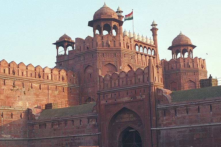
(pic source: wikimedia)

C. R. Rao was one of the early members of the renowned Indian Statistical Institute (ISI) that was founded by the legendary P. C. Mahalanobis, an institute the produces fine Operations Research grads to this day. He's briefly mentioned in an earlier post, and an upcoming post in this space will again be related to his work.

Historical Postscript
1. A story that involves covert sampling to predict the number of pro-India soldiers to provision during the 1857 war of independence in India is briefly covered in 'Operation Red Lotus'.

(pic source: http://whc.unesco.org)
2. The tomb, which was visited by President Barack Obama on his India visit, houses the mutilated remains of a so much more relevant person - Dara Sikoh, perhaps the Mughal who most deserved the suffix "great". The Red Fort (and the Taj Mahal) was built by Indian workers on the orders of Dara's father.

(pic source: wikipedia)

Dara was the most learned and compassionate in a dynasty characterized by excesses that causes resentment to this day. He respected, even celebrated the pluralism of the dharmic thought system that has defined India since times immemorial. In unbelievably stark contrast stands his brother, the fanatical Aurangazeb, who unfortunately for India, prevailed in a tense struggle for the throne and had Dara killed most gruesomely on charges of blasphemy, before proceeding to slaughter about 4.6 Million Hindus (NY Times, 2011), statistically ranking him at #23 in the all-time list of mass killers (WW2 is at #1).

June 6: edited typos.

Jugaad Innovation: Stuck in a Local Optimum

Updated July 5, 2013:
CNN link on Jugaad Innovation.

The book cover blurb sounded exciting: Do more with less. An alternative to risky expenditure-driven, resource-hungry growth using a "bottom up approach to frugal and flexible innovation". Endorsement from a salesforce.com CEO. No doubt, Jugaad is a useful concept - it's a Hindi word that implies a improvised and clever work-around, but there is such a thing as stretching an idea too far. Jugaad arises from the Indian way of doing "more with less" - possibly a public response to artificial scarcity induced by genocidal British colonization since the late 18th century when a resource-rich India's share of world GDP plummeted from 25% to a negligible quantity in a short time to turn it into from a knowledge and manufacturing economy into an agrarian, impoverished nation. A scarcity-driven economy that has been nurtured by Nehruvian socialist politics over the last 60+ years. However, the word itself ties in nicely with ideas in Operations Research that deal with the optimal allocation and utilization of scarce resources, and hence this post.

The book has some heart-warming and splendid examples of Indian innovation, which are nice to read. The remarkably decentralized and entrepreneurial nature of the workforce, and their seeming comfort in operating effectively within what appears as "chaos" to the external observer is one of the salient features of the native Indian economy. A discussion of the Indian practice of the "missed call" (the closest that mankind has come to 'half a bit' of information) adds humor. The authors could have lent depth to the book by exploring the deep-rooted cultural origins of the decentralization, and entrepreneurial spirit that drives the Indian way of doing things. They do make some useful comparisons between the profligacy and rigidity of some Western CEOs with the adaptive nature of the "jugaad entrepreneur". However, celebrating every success from Bharti airtel to PepsiCo's direct seeding to Mitticool (now that is really cool) as a win for "Jugaad" dilutes the message. When the book hyped the crappy 'Aakash' tablet, the populist, Indian government's tax-payer subsidized tablet for the unwashed masses (a cheaper and cynically sub-optimal alternative to constructing and maintaining primary schools), it was time to cry halt. Celebrating artificial scarce resource allocation, however efficiently done, feels like a cop-out.

Operations Research practice is not just about optimizing within constraints and declaring victory. Value can be unlocked by using OR to expose the more expensive bottlenecks in the system. Constraints that turn out to be artifacts must be eliminated whenever possible. I'm all for (also) 'thinking small', but not at the expense of losing the context.

Solve TRP, Drive Tesla

So the awesome and hyped Tesla Model S is beating Mercedes, BMW, and Audi in sales despite the $70K price tag. One problem is the current lack of charging stations required to recharge over long trips. CNNMoney reports:
"CNNMoney took a Tesla Model S on a test drive from Washington D.C. to Boston. The all-electric car drove 450 miles with two stops to recharge at Tesla's Supercharger stations in Delaware and Connecticut"



A second problem is that unlike conventional gasoline cars that can be refueled very quickly, charging can take a relatively long time, and adds significantly to your total travel time. In the near future, as the number of Teslas increase, the number of charging stations is likely to go up too. However, it will remain a sparse resource for some time. A future Tesla trip from New York to California will require many recharging stops, reminiscent of the old stagecoach problem during the Gold Rush era, which is used to illustrate the principles of Dynamic Programming.

Update: May30, 2013
Popular Mechanics reports:
"...the California-based EV automaker plans to expand its fast-charging "supercharger" network across the continental U.S. During today's announcement, Musk said New York to Los Angeles trips would be viable as soon as this winter. 

"When you get in a car you have the ability to go almost anywhere," Musk said. "That's what the supercharger network will do." 

The rollout will begin as soon as this summer, with the number of stations tripling to 27 nationwide by the end of June. In addition to increasing supercharger density along the already-established California and Mid-Atlantic coasts, Tesla will debut chargers in a handful of new metropolitan areas within the next few weeks, including Austin/Houston, Portland/Seattle, Boulder/Denver, and Chicago/Milwaukee. By the end of the year, Musk expects to to have "a couple hundred" superchargers spread across the U.S. and southern Canada, with as little as 80 to 90 miles between stations along the Altantic and Pacific coasts..."

Tesla Routing Problem
Given a road network G having a limited number of charging stations located at specific nodes, the Tesla Routing Problem (TRP) will have to:
Find the shortest feasible time path from origin O to Destination D in network G.

Feasibility requires the car to visit enough charging stations in a timely manner. Optimality requires that the sequence of visits be carefully selected such that the total time spent is kept to a minimum.

Total travel time = driving time + recharge time

This involves two decisions:
D1. Which recharging stations to visit en-route?
D2. How long to recharge at every pit stop?

Assumptions:
A1. The longer you recharge, the longer your available range (to a limit).
A2. All recharging stations are similar, and infinite capacity (no queuing!)
A3. Range is deterministic

Update on A2: The Tesla can charge on any outlet, but the time to recharge can vary depending on the source.

Clearly, optimally solving TRP involves the finding a solution to a Traveling Salesman Problem even in the special case of instantaneous recharge (Y=0).

(Updated September 2013: As mentioned in the comments, the general case is not a TSP in the network of charging stations. Here, the assumption is that stations are sparsely located and we visit each one along the way. The title is changed to reflect this distinction).

This is no different from the (milder) challenge faced by conventional car drivers in unfamiliar areas where gas stations may be hard to come by (see this old post). Charge cannot be carried in Jerry-cans. The  shortage of charging stations does make every long Tesla trip a non-trivial problem to manage. Tesla owners have to deal with a NP-Hard Optimization Problem (Heh) on every such trip, but in practice, it should not be difficult to find good quality, feasible TRP solutions.

The recharge time makes the TRP a bit more interesting. If two stations are close to each other, we don't have to recharge fully, and just need the minimum to reach the next stop - or perhaps we recharge fully, which allows us to reach a station that is further away but turns out to be more time-effective, overall. Clearly, these two decisions appear to be interlinked and may need to be jointly optimized. D1 is a binary decision variable X(i) - we either visit or don't visit a station at node X(i), whereas D2 is a semi-continuous variable Y(i) conditional on D1:

Y(i) ≤ U.X(i)
where U = maximum recharge time.

Another interesting and maybe even useful problem for Tesla-makers to solve is where to add new charging stations on the network G over time. What is the minimum number and location of stations required to guarantee feasible solutions to any TRP in the 48 states of continental US? How will stations deal with congestion in the future? and so on ...

I haven't driven a Tesla yet but I wouldn't mind relocating my office to inside one and telecommute.

Guesstimation in Optimization and Analytics

Guesstimation
Browsing through the various examples examined in the 2008 book 'Guesstimation', it is apparent that the basic ideas behind this approach of "solving the world's problems on the back of a paper napkin" are useful for analyzing real-life optimization and analytics instances. Whether we are looking at (i) Smart-grid optimization ("how many hours does it take to charge an electric car"), or (ii) Hazmat routing ("what is the risk of dying per unit mile of road") or (iii) environmental problems ("how much farmland will it take to convert all gasoline cars to ethanol"), guesstimating values can be critical to effective model formulation in the absence of precise information. Guesstimation is a 'small data' method that can improve the effectiveness and performance of our 'big data' analytics.

Optimization
Let's look at an 'elastic' linear programming formulation:
LP: Minimize c.x + P.s
A.x - s <= b
l <= x <= u, s >= 0
where we've added artificial variables 's' to ensure feasibility of LP for any bound feasible 'x'. Often times, exact values for b, c, l, u, or portions of A are not available. Furthermore, we allow artificial variables to be active at some high but as yet unknown penalty rate of 'P'. We often end up guesstimating these values in industrial applications since many of these values are not known accurately.

Example (i) in the previous paragraph gives us a charge rate per car (a component of 'A' matrix). if 'x' is the number of cars to be charged, and 'b' is an upper bound on the time available and 'c' the cost of electricity for that duration, we can predict the 'ballpark' cost incurred and the charge stored. Similarly, example (ii) gives us the average risk per unit mile as a cost coefficient 'c'. By extending this calculation to denote high and low risk arcs in a network, we have an initial minimum risk network path optimization formulation at hand. Finally, example (iii) gives us an unconstrained resource requirement. This value allows us to quickly assess the impact of adding a resource constraint.

Thou shalt always Guesstimate!
Direct uses of guesstimation in practical optimization include the calculation of tighter bounds (l, u) for decision variables, and the smallest valid values for the big-M numbers that riddle integer programming formulations. If we think of (u - l) as a measure of our ignorance about the as yet unknown optimal 'x', guesstimating tight bounds is akin to maximally reducing its "prior variance". While guesstimation in the book is done using feasibility calculations, we can and should incorporate optimality considerations to obtain sharper bounds for such unknown variables. Using solver default (0, infinity) values is lazy and bad practice. Also, spending some time to improve bounds often gives us insight into the nature of the optimal solution, and which constraints are likely to be more restrictive, and helps catch modeling bugs earlier.

Example 1: what is the cost of not scheduling a crew for an airline flight?
In airline crew scheduling, the flights in a schedule are partitioned among crew pairings (see this post for a problem description). Every flight must be covered by exactly one pairing. This is a hard constraint, but in practice, we have to temporarily employ its elastic form of the type described above, and penalize violations via 'P'. How do we determine an appropriate penalty value? This would be the cost of leaving a flight uncovered. Such flights have to be covered by a reserve crew, which comes at a certain cost that can be calculated and is typically smaller than some default value we may have otherwise chosen. The dual variable value associated with an uncovered flight in an optimal LP solution attains a value close to 'P'. Any new column (x(j)) generated that covers this flight will subsequently will have a reduced cost of order (c(j)-P), and so on. Good guesstimation of P helps in producing manageable reduced costs, and accelerates algorithm convergence.

Example 2: what is the price elasticity of point-and-shoot digital cameras?
Price elasticity is a dimensionless (negative) quantity that gives us the expected percentage change in sales for a percentage change in price. We can expect that this value will be more than that for electricity, grocery, and dairy items, which are essential items that people are less willing to give up when price is hiked, and are likely to be inelastic (less than a percent drop in sales for a percent increase in price, say -0.5). The value will be lower than that of highly discretionary purchases like fashion apparel or leisure airline tickets (which have an elasticity of -4 to -2). The geometric and arithmetic mean of 3.0 and 0.5 gives us a range (-1.8, -1.2). A data-driven estimation of this value should be compared against this guesstimate as a sanity check. For example, if regression models on a data sample estimates an 'optimized' elasticity parameter value of -5 or -0.1, we may want to double check our modeling, or run the risk of producing wild predictions.

Another use of guesstimation is in generating plausible random optimization instances to demonstrate the effectiveness of new NP-Hard algorithms for a certain problem class if only limited real-life data is available. It can help weed out weird and contrived instances that skew the degree of difficulty of the problem and make it seem much harder than it actually is in reality.

Fun with Coins: Optimizing The OR Cafe Price Menu

We've looked at a few coin-optimization models here before. ... We'll look at another one today. We'll try to price the menu at OR cafe. You can look at the detailed problem statement and the associated sample data here. As always, there's no claim that the method described here is a 'best' or even a 'correct' way to manage such a problem. This post serves as a useful starting point for analyzing this fun problem with coins and change.

Basically, the problem we are analyzing in this post here is to change the existing prices of items in the menu by tiny amounts (+/- 2 cents) to maximize the number of (future) customer bills that end with zero or five cents (i.e., $x.05, $x.10, $x.15, ... $x.95) after (13%) tax. Assuming that past transactions (200 of them) are a good indicator of future purchase patterns, we can select a portion of this data (say 60%) to 'train' our pricing model (MIP) on, and then evaluate its performance on the remaining 40% of the transactions.

Model
1. Decision variables: There are five pricing possibilities for the recommended price of an item p(i) = {p0(i)-2, p0(i)-1, p0(i), p0(i)+1, p0(i)+2}, where p0(i) = original price of the item in the menu.

2. Bill(transaction j) b(j) = sum(i) Aij.p(i)*(1+T/100)
where:
a. Aij = number of units of item (i) purchased in historical transaction (j)
b. T = percentage sales tax charged

3.The minimum (l(j)) and maximum (u(j)) values for b can be determined by setting all prices to their lower bounds, and upper bounds respectively. We assume that fractional cents are rounded to the nearest cent. This gives a pre-computable range of feasible b values V(j) = {l(j), l(j)+1, ...., u(j)}.

4. Objective: Maximize the number of times b ends in 0 or 5 (using boolean indicator variable 'z' and 0-1 cost 'c') in the training set by selecting one price from the 5 possibilities for each item

CAFEMIP: Max sum(k,j) c(k,j)z(k,j)
subject to:
ii)  sum(i) Aij.p(i)*(1+T/100) = sum(k)V(k, j).z(k, j) for all j
iii) SOS-1 constraints for: prices p(i) that ensure that one of five prices is picked for each item in the menu, and for z(j) to ensure that exactly one bill realization is active for each transaction.

Round-off Issue
The LHS of constraint 4(ii) can contain fractional cents, whereas the RHS only admits discrete values. This situation can be overcome as follows:
b(j) = sum(i) Aij.p(i) + sum(i) Aij.p(i)(T/100) = b'(j) + tax,
where b'(j) is integer. Every realization of b'(j) (=V'(j)) can be mapped to our 0-1 objective function contribution after accounting for the additional tax it generates. Thus, it is sufficient to retain the integer components of 4(ii) and rewrite it free of round-off error as:

sum(i) Aij.p(i) = sum(k)V'(k, j).z(k, j) for all j

CAFEMIP was optimized using CPLEX 12.x and implemented in Java. As a secondary objective, a tiny penalty was added to minimize the deviation of prices from the original value to avoid unnecessary price changes or revenue shifts.

Results
1. optimized over the entire 200 transactions (no hold-out sample).We count the number of times, the cafe needed to round to the nearest 0 or 5 using the prices before and after optimization.

Roundings needed: original price:   135/200
Roundings needed: optimized price: 35/200
While the results on training data are really good, we do not know how well CAFEMIP would do on hidden data, so we re-run CPLEX on a subset of the data.

2. Optimized over the first 120 transactions only, and tested on the last (hidden) 80 transactions.
training data: original  cost =     77/120
training data: optimized cost = 20/120

--- CPLEX log ----

Tried aggregator 1 time.
MIP Presolve eliminated 34 rows and 17 columns.
Reduced MIP has 230 rows, 847 columns, and 1824 nonzeros.
Reduced MIP has 835 binaries, 0 generals, 0 SOSs, and 0 indicators.
Probing fixed 68 vars, tightened 0 bounds.
Probing time =    0.01 sec.
Tried aggregator 1 time.
MIP Presolve eliminated 4 rows and 207 columns.
MIP Presolve modified 14 coefficients.
Reduced MIP has 226 rows, 640 columns, and 1666 nonzeros.
Reduced MIP has 629 binaries, 11 generals, 0 SOSs, and 0 indicators.
Presolve time =    0.06 sec.
Probing time =    0.02 sec.
Clique table members: 3071.
MIP emphasis: balance optimality and feasibility.
MIP search method: dynamic search.
Parallel mode: deterministic, using up to 4 threads.
Root relaxation solution time =    0.00 sec.

        Nodes                                         Cuts/
   Node  Left     Objective  IInf  Best Integer     Best Node    ItCnt     Gap

      0     0       13.3095    48                     13.3095       92         
*     0+    0                           73.0000       13.3095       92   81.77%
      0     0       18.8333    13       73.0000     Cuts: 130      189   74.20%
      0     0       20.0000     2       73.0000      Cuts: 22      220   72.60%
*     0+    0                           20.0000       20.0000      220    0.00%
      0     0        cutoff             20.0000       20.0000      220    0.00%
Elapsed real time =   0.16 sec. (tree size =  0.00 MB, solutions = 2)

Clique cuts applied:  34
Cover cuts applied:  35
Implied bound cuts applied:  4
Mixed integer rounding cuts applied:  7
Zero-half cuts applied:  7
Gomory fractional cuts applied:  28

Root node processing (before b&c):
  Real time             =    0.09
Parallel b&c, 4 threads:
  Real time             =    0.00
  Sync time (average)   =    0.00
  Wait time (average)   =    0.00
                          -------
Total (root+branch&cut) =    0.09 sec.
CPLEX objval = 20.000000000000025

original, new price of XS Coffee is $1.24, $1.24
original, new price of S Coffee is   $1.33, $1.33
original, new price of M Coffee is   $1.57, $1.55
original, new price of L Coffee is    $1.71, $1.73
original, new price of XL Coffee is  $1.91, $1.90
original, new price of S Tea is        $1.33, $1.32
original, new price of M Tea is       $1.52, $1.51
original, new price of L Tea is        $1.71, $1.73
original, new price of Donut is       $0.95, $0.97
original, new price of Bagel is        $1.24, $1.24
original, new price of Muffin is       $1.30, $1.28
original, new price of Cookie is      $0.75, $0.75


(prices in red indicate a changed recommendation when optimizing over the partial sample instead of the entire history)

These prices were used to recompute the bills in the hidden sample:
hidden data: original  cost =   58/80 (~72%)
hidden data: optimized cost = 17/80 (~21%)
Thus, we would have been able to significantly reduce the number of roundings on the hidden sample if we used the CAFEMIP prices instead of the original values. If the customer buying pattern remains the same, we can expect these prices to continue to do a good job. 

Optimally Managing Ladybugs

My daughter loves ladybugs.  However, when it comes to cleverness, many have noted how bees and ants (which seem to have a special place in Indian hearts :) "solve" traveling salesman and shortest path instances that matter to them (see this interesting link as well). In contrast, a ladybug's decision analytics appears to be somewhat shaky. They don't seem to have the kind of auto-GPS of bees and ants (at least in the context of this post), and seem to get confused and stray from their optimal path.

(pic source)

Recently, a number of LBs invaded my residence, and I spent a lot of time trying to shoo them away and determine how they got inside in the first place so that I could block their entry. Then, I came across this website. Apparently, ladybugs prefer humidity and warmth and try to enter homes as winter begins. OK. However, a good number also enter the house come spring time, which was puzzling. It seems some of the LBs goof up. Ladybugs roosting under windows outside the house, with a certain probability, enter the house instead of enjoying spring time outside. Once inside, they suffer from dehydration and die (unless they figure out the route to the bathroom or kitchen). If we try to force them out, they get stressed and shed 'yellow blood' that can stain walls. The optimal ladybug solution for this time of the year is to simply open the windows, so the ones who came inside by mistake can leave. It's a win-win for both parties, and it actually worked. On the other hand, during winter, we have to try and provide a cozy, alternative home in backyard and insulate the house well to keep them out.

The "Chaos" of India

Thanks to the person who pointed me to an interesting article in some online magazine called "livemint" : "Why Rahul Gandhi has understood the chaos of India"

As the 2014 General Election in India approaches, and pro-establishment journos crank out essays defending their favorite candidates, the author of the above article attempts something truly brave: resurrect a universally panned speech by a leading politician of the incumbent ruling political party. In particular, this paragraph caught my attention:
"... There are two things that stand out in the speech. The first is Rahul’s recognition of the chaos of India, for which he used the image of the beehive. I think this is wonderful realism, and excellent imagery."

As a keen India observer and commentator pointed out on twitter: "....beehive is nt chaotic"

Is India really chaotic?
To many a visitor from the west, it has appeared so. A vast section of India's English media who have worshiped at the altar of Western Universalism and return to lecture India's unwashed masses, may readily concur.

India, for a long, long time, has functioned as a highly decentralized system - in virtually every aspect of life. It's workforce contains among the highest percentage of entrepreneurs in the world, and traditionally possesses a remarkably decentralized economic model. It's indigenous religions are decentralized and base on empirical self-realization. There is no single holy book or authority (there is an entire reference library, with scope for new books to be written). However, this lack of a central authority does not imply chaos or that India was never a nation. It is more likely that what is perceived as chaos is in fact a cognitive overload on the part of the casual observer - as noted in Rajiv Malhotra's book "Being Different". The best example for this apparent chaos that actually produces incredibly effective results is the Kumbh Mela (the largest human gathering on earth, which has been recurring for thousands of years now) that recently concluded in India. Several observers from Harvard and other big-brand western institutions showed up this time to analyze this amazing event. Here's what Rajiv Malhotra says about the Mela:

"....India's Kumbha Mela amply demonstrates that diversity can be self-organized and not anarchic, even on a very large scale. Held every twelve years, this is the world's largest gathering of people, attracting tens of millions of individuals from all corners of India, from all strata of society, and from all kinds of traditions, ethnicities and languages. Yet there is no central organizing body, no 'event manager' to send out invitations or draw up a schedule, nobody in charge to promote it, no centralized registration system to get admitted. Nobody has official authority or ownership of the event, which is spontaneous and 'belongs' to the public domain. Since time immemorial, numerous groups have put up their own mini-townships and millions go as individuals just to participate in the festivities."

How and Why? Rajiv argues in his introduction to the chapter "Order and Chaos":
"Indians tend to be more relaxed in unpredictable situations than westerners. Indians indeed find it natural to engage in non-linear thinking, juxtaposing opposites and tackling complexities that cannot be reduced to simple concepts or terms. They may be said even to thrive on ambiguity, doubt, uncertainty, multitasking, and in the absence of centralized authority and normative codes. .... In the vast canon of classical writings in Sanskrit, we see many context-sensitive and flexible ways of dealing with chaos and difference. The search here is always for balance and equilibrium with the 'rights' of chaos acknowledged. On the other hand, in the creation stories in Genesis and in the Greek classics, there is a constant zero-sum battle between the two poles in which order must triumph."

Interestingly, the socio-biological systems of beehives and ant colonies, which may appear chaotic to the casual observer has an underlying order. In his brilliant book 'Traffic: why we drive the way we do', Tom Vanderbilt quotes studies that note how vast numbers of ants move without colliding (without a centralized traffic cop ant), which is certainly worthy of emulation by human car drivers. The author notes "looking at the swarm as a whole, one might not see what is driving the movement". The insects have their own Kumbha Mela going, perhaps.

Rahul Gandhi's 'beehive' metaphor may not be unreasonable, but it appears to have been chosen based on an entirely shallow reasoning due to his inability to decipher India's apparent "complexity", which he contrasts with China's 'simplicity'. India can be plausibly compared in certain contexts to a beehive or an ant colony not because of 'chaotic frenzied activity', but because of an certain well-functioning harmonic order underlying the apparent chaos.

The lesson here for those of us wishing to properly study India is to look beyond the obvious, look deeper, pay attention to context, and there are amazing discoveries waiting to be made. When Rahul Gandhi, the 4th edition of the Nehru dynasty and potential contender for the post of prime-ministership in 2014 compares India to a beehive for all the wrong reasons; when sections of the Indian English media jump in to spin this into some 'deep thought', it only betrays a fundamental lack of understanding of the essence of India: pluralism, diversity, and cooperative decentralization, blissfully unaware that at its deepest philosophical levels, dharmic India is bound by what Rajiv Malhotra terms an 'Integral Unity'.

Synchronized Scheduling Case Study - Part 3

The case study is introduced here.
The ICAR goal is derived here.

Model
The ICAR problem can be specified as follows:
Find a set of feasible crew pairings and aircraft strings such that:
a. every flight in the LEG schedule is covered exactly once by an aircraft string

b. every flight in the LEG schedule is covered exactly once by a crew pairing

c. any string and pairing is used no more than once (let's denote the non-zero pairings and strings as 'active')

d. the total cost is minimized

e. if an active crew pairing contains a connection t(i→j) in T, and there is also some active aircraft string that also contains t, then we say that the crew turns with the aircraft and is thus synchronized. Downstream systems can ensure that the actual crew assigned to flights i and j remain with the actual aircraft tail number that flies i and then j.

f. Maximally satisfy a reliability measure that is proportional to the tightness and the number of the synchronized connections in T. For the purpose of illustration in this post, we specify that a certain minimum count (m) of the connections in T be synchronized. The aim here is to be smart about picking the right airports and connections to synchronize to boost reliability as well as utilization.

g. The active strings belonging to a sub-fleet should form a Hamiltonian circuit. This is a maintenance requirement that tries to ensure equal wear-and-tear across the fleet. There are other constraints that are also interesting topics in their own right, but we'll ignore them here for brevity.

Resource Synchronization Modeling
Our main focus here is on requirement (f). We provide some sample approaches to handling synchronization in large-scale scheduling:
a) Within the subproblem: 
Really tight day-connections t in T can be directly enforced by restricting t to be the only valid connection out of i and into j (i→j) in the flight network. Thus any pairing or string that comes of the subproblem that covers flight i will subsequently cover j. However, we cannot apply this  idea to all connections in T since that is likely to be overly restrictive. 

b) Within the Master program: 
Let p(t)  = sum of all pairing variables that contain connection t
q(t)  = sum of all string variables that contain connection t
Note that p and q will be no more than 1.0. We can impose the following synchronization constraint: 
∑_T p(t)q(t) ≥ m 



The bilinear terms in the reliability constraint can be linearized in a straightforward manner. A personal favorite is the reformulation-linearization technique (RLT). z(t) ≡ p(t)q(t) ⇒

∑_T z(t) ≥ m, z(t) ≤ p(t), z(t) ≤ q(t), z(t) ≥ p(t) + q(t) - 1

Thus, by adding O(T) very sparse constraints and continuous variables z, we can model the synchronization component of ICAR without requiring any approximation, and the resulting formulation remains tractable. The RLT can be applied in a similar manner to synchronize three or more resources as well. The keys for this 'frontal assault' to work are:
1. The cardinality of set T be manageable in the context of the application.
2. Synchronizing two resources is easier than juggling three or more. We can see from the synchronization constraint that if the p-variables are fixed, the z-variables can be eliminated, leaving us with just the q-variables. This 'two variable per constraint' structure makes life much easier during column generation. The synchronization duals associated with the connections in T tend to work much more effectively in generating string-pairing pairs that cover a beneficial subset of common turns in T.

Epilogue

The ICAR solutions that were actually implemented (different from the illustrative version presented here) significantly improved upon the existing approach. It reduced business cycle time, greatly increased reliability, and reduced costs. The success of the ideas employed to tackle ICAR spurred the development of new, algorithmic techniques to solve the next-generation integrated crew scheduling problems that went on to save the LEG carrier many million bottom-line dollars annually during some difficult economic times. As far as the competition with LCA was concerned (for which this solution was designed): LEG had incurred enough losses and pulled the plug. Operations Research successful, patient dead.

Synchronized Scheduling Case Study - Part 2

The case study was introduced in the previous post. Read the introduction here.

.... Despite their suboptimal approach, the schedulers of the LEG carrier did some nice work with their synchronization approach.

2SAT versus 3SAT
There is a jump in decision complexity when moving from a two-body conflict resolution problem to three-body conflict-resolution. Intuitively, we can observe this in linear programming (LP) problems. LPs limited to two variables per constraint are easier to solve. The dual (two constraints per variable) is a generalized network flow problem that can be solved using purely combinatorial methods. Intuitively, one can adopt an alternating heuristic that iteratively fixes one variable and optimizes the resulting univariate problem. In computational complexity theory, SAT-2 is easier to manage compared to SAT-3.

Rather than trying to simultaneously juggle flight attendant (FA), pilot, and aircraft maintenance schedules, the LEG schedulers adopted an simplification. They combined the two human elements into a single 'crew' scheduling entity. This can be achieved via "co-pairing", i.e., by building common pairings (partial schedules) for FAs and pilots employing X = {X_PILOT ∪ X_FA}, i.e., every pairing would be feasible to both pilot and FA contracts and FAA regulations. Column generation allows you incredible flexibility in accommodating such a change. This flexibility is invaluable when hit by a perfect storm. Now, they could work with a two-variable per constraint structure so that their telephonic "alternating heuristic" negotiations could converge in a timely manner. Unfortunately, such a beneficial reduction in complexity was accompanied by inefficiency. The approach erred inordinately on the conservative side. The resources were now too tightly integrated, resulting in a cost spike due to under-utilization of expensive resources. LEG's R&D team was invited to resolve this problem.

Integrated Crew and Aircraft Routing (ICAR)
The OR team quite naturally proposed an integrated scheduling approach that would reduce costs, improve reliability of operations, and also enable tactical synchronization of flight connections. However, the number of possible connections to be evaluated is O(n²) for a n-flight schedule. Methods in the literature are typically data-agnostic; sophisticated alternatives to the straightforward approach designed to perform an acceptable job even in the worst case. Luckily, LEG's OR team had to solve only LEG's problem and not that of every future airline and space shuttle.

The Beauty and the Brute Force
Given the problem size spread over a five-day period, there are a few million candidates to synchronize in the theoretical worst case. However, our focus is only on same and overnight connections, which reduces the candidate list to a few hundred thousand. When we recognize that we only have to focus on the set T of connections of the same sub-fleet type at the same airport (duh), and exploiting a few other contextual restrictions, this final number is data-driven. It turned out that there were no more than tens of thousands of synchronization possibilities to deal with, 99% less than the theoretical bound. This finding allowed the possibility of cheerfully discarding (as we found out a couple of years later when some of the first journal papers on ICAR came out) all the neat out-flanking theorems and approximations presented in the literature.  The method chosen may score low on aesthetics but was effective and flexible in managing the full blown ICAR instances in context. There is a childlike joy in discovering that enumeration solves your practical business problem - akin to finding out that this emperor has very little clothes. This basic counting step gave the team a clear goal.

Problem Statement (at last)
Given a flight schedule, jointly construct feasible crew pairings and aircraft strings such that their scheduling intersection (elements within the connection set T) are optimally synchronized.

And, yes, there were a few TSP (Traveling Salesman Problem) instances to be managed within ICAR. To be continued....

Synchronized Scheduling Case Study - Part 1

Synopsis 
When a low-cost airline (LCA) entered a short-haul aviation market many, many years ago, a legacy airline carrier (LEG) decided to compete with LCA on its own turf by matching the LCA's fare, frequency and super-quick aircraft turn-around times on ground ('turns' for short). This required a high degree of coordination between LEG's in-flight crews (pilots and flight-attendants), ground-crew, airplane maintenance planners, and the airline schedulers (including their scheduling optimization system). In particular, the utilization of the pilots and the flight-attendants had to be maximized. The challenge however was that all these different resources were part of separate organizational structures and were governed by different contractual rules, and the LEG idea eventually turned out to be cost-prohibitive and unreliable due to poor synchronization of resources.  On the other hand, the Operations Research (O. R) team built a specialized scheduling system for LEG (far ahead of the literature available at that time) that would've achieved the needful. Unfortunately, the silo-ed organizational structure hindered adoption.  Result:  Unlike the legendary revenue optimization contest where the legacy carrier triumphed, the tables were turned here, and the LCA flourished. The low-cost LEG idea was resuscitated many years later in a different context and market, and did a better job using the lessons learned from this early setback. In the next few posts, we will compare the two approaches used to synchronize these resource scheduling tasks and summarize the lessons learned.

Airline Scheduling Basics
Given an aircraft schedule, the resource planning is done sequentially in order of their profitability (or cost) to the airline. Thus:
LEG flight schedule → pilot schedule→ flight attendant schedule → aircraft maintenance routing

The cost-critical task here is the construction of "pairings" (or "strings" for aircraft), which denote partial (unassigned) solutions that represents partial tours of a resource. For LEG pilots (set of two persons), and FAs (set of three persons), this represents a tour in a time-space network that starts from a crew domicile (a small subset of airports in the LAC schedule), traverses a bunch of different airports over 1-5 duty days with intervening periods of rest known as layovers, before returning to the home domicile, while satisfying a myriad of contractual and FAA rules for work hours, rest time, etc. In short, the cost and constraints that determine each pairing is an extremely complicated nonlinear, non-smooth, non-convex, nonplussing mixture of on-duty + rest + reliability + crew work life balance + other path-dependent factors. 

Good quality pairings can be created using a dynamic column-generation procedure. A column here represents a pairing, and during an optimization run, thousands of pairings are generated and selected from among the many trillions of possibilities using a "branch and price" scheme. Eventually a subset of the generated columns are selected such that every flight in the time-space network is covered by exactly one pairing, and such that the total cost is minimized (where the actual 'cost' being optimized is a combination of a hundred-odd objective function components).

Note: An airline crew-pairing solver's set partitioning problem is arguably the easiest optimization model in the world to represent on paper:
{SPP: Minimize cx : Ax = 1, x binary, x ∈ X}

In contrast, the real-life computer code used to manage this simple model can easily run in the order of many hundred thousand lines (largely due to the complicated and detailed nature of X), with expensive parallel-processing machines, and an embarrassment of CPLEX licenses to match. Why? A small percentage point reduction in crew pairing cost (cx) can easily recover all these infrastructure costs and then some. Since crews get paid the max of planned and actual costs, these numbers are actual bottom-line savings. Furthermore, such scheduling tools can be mission-critical systems that run 365 days a year, requiring O.R product support staff to be on call like primary care doctors. 

Solution Approach
Downstream systems, and not of immediate interest to this post, combine these pairings into actual monthly schedules with pilot, first officer, and flight attendants assigned by solving yet another set-partitioning problem. Thus cost-effectively scheduling even a single resource requires a sophisticated solution approach. In those days, academic literature often contained interesting approaches that looked good on paper but proved to non-implementable because of the highly context-driven and data-driven nature of this problem that requires developers to pay careful attention to problem size, exploit special structures in SPP and X, and keep in mind certain carrier-specific objectives. On the other hand, interested readers can refer to this journal paper - the first one I read on the job. It is also the #1 cited INFORMS paper based on a recent ranking. Today, this portion of airline planning is typically outsourced to specialized airline crew-scheduling software vendors.

Pairings and Strings
A set of pilot pairings tell you, for any given LEG flight: the in-bound flight that the pilots arrived in, and the out-bound flight on which they will depart. Of course, if a LEG flight schedule is built with lots of tight turns (say 30 minutes or less) at an airport, then it makes sense from the point of view of operational reliability and cost, for the crews to stay with, and depart on the same airplane, assuming of course, that the aircraft routers will assign the same aircraft (tail number) to these flights. This is a resource synchronization rule: Keep crews and aircraft together to the extent possible while also keeping costs low and satisfying all contractual duty, rest, and maintenance rules.

The FA scheduling system can take pilot pairings as inputs to try and keep the FAs with the pilots. Unfortunately, since these crews have different operating hours and safety rules give the varying nature of their job descriptions, very often, pilots and FAs have to break up and depart on different flights. This is an operational nightmare when you are trying to work with tight turns to compete with LCA, and actual costs shoot up if you 'over-synchronize'. To make matters worse, the strings (partial aircraft maintenance routing solutions) also have to be tightly woven with crew pairings. It's a planners nightmare.  Believe it or not, LEG folks actually built much of these schedules separately ("legacy approach"), with each scheduler anticipating what the other person will do, often coordinating via phone-calls in this multi-person game. Result: an expensive and sometimes operationally brittle schedule that increased operational costs and ate up some customer goodwill, which eventually resulted in the plug being pulled. In the next part, we'll see how LEG's OR team analyzed this problem.

to be continued .....