More specifically, the fear of having to solve an NP-Hard optimization problem to save your job.
Do you or anyone else in your organization exhibit symptoms of Ekthetikophobia?
Sample Responses by Ekthetikophobes
1. Resign: Capitulation is by far the most common response, especially if the person does not have an ORMS background and is oblivious to the 'science of better'. Throw hands in the air, lose faith in humanity, and slurp spoonfuls of the nearest meta-heuristic algorithmic prescription provided by bees, ants, bacteria, squeaky wheels, mutant turtles, ... any nature cure that uses pseudo random numbers. This response is best captured by the Hindi proverb "Naach Na Jaane, Aaangan Teda",i.e., a bad dancer blames the uneven floor.
2. Controlled Panic. This is pretty typical of a generation of OR practitioners weaned on CPLEX. Like MDs trying to decode a deadly new strain of flu, the overriding urge is to throw money at the problem by ordering the latest versions of the baddest bunch of industrial strength optimization solvers in the market with matching supercomputing accessories to run massive benchmarks, and generally scare the pants off their IT managers who work with depression-era budgets.
3. Code. This is relatively more common to programming gurus and follows exactly one rule: If you throw sufficiently well-written code at any problem, it must work. This is so crazy, these guys are on to something here.
4. Publish. The median response from E.phobic research folks is to put this exhibit on a pedestal for everybody to gaze at. It's akin to a biologist discovering a new specie or an astronomer sighting a new planet that shouldn't have been there. Half of these people (surely OR types) will go on to demonstrate the monstrosity of this new problem based on diabolical worst case instances that even a God who plays dice would not inflict on mankind. The other, more elegant half (theoretical CS E.phobes) propose 'factor of 2' approximations that cover all remaining difficult instances missed by the Muggles, yet just as useful practically, before declaring victory. Then over the next two decades: keep shaving of that factor; rinse & repeat; it's a veritable cottage industry.
Exaggerations aside, ranked at the top of the most systematic, resourceful, innovative, and practically useful responses toward 'new' NP-Hard optimization problems must be the approach adopted by Dantzig, Fulkerson, and Johnson (1954) to tackle a 49-city Traveling Salesman Problem using 1950s computing technology and fearless minds that dared lasso the exponential.
July 22: minor fix: added missing text.
Sunday, July 22, 2012

Thursday, July 19, 2012
Predicting the Value of a Bunch of Coins
This is the last part of the 'Coin trilogy'. Here's part-1 and part-2. In this post, we attempt to answer questions on predicting the value for a bunch of coins for which we only know its weight but not the exact internal distribution among coin types.
If somebody gave you the option of choosing either the value of a kilo of coins or 40$, which will you pick?
Using CPLEX, we determine that the maximum possible value for 1000 grams of pennies, nickels, dimes, and quarters is 44.05$, so if you took the 40$, there is a small chance you will incur a loss. If the bag was packed with 400 pennies (weighs exactly a kilo), you'll make a 36$ profit. If the coins types were uniformly distributed, its value would be about 26$, and you would make a 14$ profit.
Say you believe you have 100$ worth of coins in a jar that you want to cash out at a Coinstar machine. How much would that weigh? A lower bound for that answer is 2.268 Kilos. If the coin types were uniformly distributed in the jar, you would carry about 3.7 Kilos.
What kind of coin ratios does a vending machine carry? This online post author made enough purchases to empty out a vending machine and found this:
Quarters:Dimes:Nickels in the ratio 1:2:1.175
Assuming that the vending machine has to satisfy exact change for any value between 5c and 95c in 5c increments, a minimum weight solution is:
Nickels:1, Dimes:9 (10 coins, weight 25.412g) with zero quarters. However, by adding a secondary objective of also minimizing the number of coins (limited coin capacity?), we obtain the following alternative optimal solution that threw away 5 dimes and picked up 2 quarters:
Nickel:1, Dime:4, Quarter:2 (7 coins, 25.412g)
Quarters and Dimes are now present in the same ratio as that in the vending machine. However, our model doesn't like nickels much (although a melted nickel was once worth more than its value).
I have a digital counting jar that displays the current value of the coins currently in the jar. It currently reads $20.05, and its weight (excluding the empty jar) is about 700 grams. For this weight, the maximum value is 30.85$. If my coins were uniformly distributed in the jar, the model predicts a "maximum" value of 18.7$, which means that I have relatively more dimes and/or quarters in my mix. A dime and a nickel have the exact same bang-to-buck ratio, i.e. value/weight ratio, which is a source of the alternative optimal solutions discussed in part 2.
US Mint Production
Averaged over 2010-2011, the coins are produced in the approximate ratio:
p:n:d:q
12:1.5:3.5:1
Quite different from our preferred ratios calculated in part-1 and part-2. At this rate, my 700 gram jar would contain only about 15$ and a kilo of coins in this ratio would be worth about 18$.
If somebody gave you the option of choosing either the value of a kilo of coins or 40$, which will you pick?
Using CPLEX, we determine that the maximum possible value for 1000 grams of pennies, nickels, dimes, and quarters is 44.05$, so if you took the 40$, there is a small chance you will incur a loss. If the bag was packed with 400 pennies (weighs exactly a kilo), you'll make a 36$ profit. If the coins types were uniformly distributed, its value would be about 26$, and you would make a 14$ profit.
Say you believe you have 100$ worth of coins in a jar that you want to cash out at a Coinstar machine. How much would that weigh? A lower bound for that answer is 2.268 Kilos. If the coin types were uniformly distributed in the jar, you would carry about 3.7 Kilos.
What kind of coin ratios does a vending machine carry? This online post author made enough purchases to empty out a vending machine and found this:
Quarters:Dimes:Nickels in the ratio 1:2:1.175
Assuming that the vending machine has to satisfy exact change for any value between 5c and 95c in 5c increments, a minimum weight solution is:
Nickels:1, Dimes:9 (10 coins, weight 25.412g) with zero quarters. However, by adding a secondary objective of also minimizing the number of coins (limited coin capacity?), we obtain the following alternative optimal solution that threw away 5 dimes and picked up 2 quarters:
Nickel:1, Dime:4, Quarter:2 (7 coins, 25.412g)
Quarters and Dimes are now present in the same ratio as that in the vending machine. However, our model doesn't like nickels much (although a melted nickel was once worth more than its value).
I have a digital counting jar that displays the current value of the coins currently in the jar. It currently reads $20.05, and its weight (excluding the empty jar) is about 700 grams. For this weight, the maximum value is 30.85$. If my coins were uniformly distributed in the jar, the model predicts a "maximum" value of 18.7$, which means that I have relatively more dimes and/or quarters in my mix. A dime and a nickel have the exact same bang-to-buck ratio, i.e. value/weight ratio, which is a source of the alternative optimal solutions discussed in part 2.
US Mint Production
Averaged over 2010-2011, the coins are produced in the approximate ratio:
p:n:d:q
12:1.5:3.5:1
Quite different from our preferred ratios calculated in part-1 and part-2. At this rate, my 700 gram jar would contain only about 15$ and a kilo of coins in this ratio would be worth about 18$.
Tuesday, July 17, 2012
Alternative Optimal Solutions to the Coin Mix Problem
The solution to the 'optimal change' problem analyzed in the previous post is further examined from a practice perspective. Again, we use CPLEX to do this since it is quite convenient for such analyses.
Problem 1 is an integer knapsack problem that is known to be theoretically NP-Hard but fairly easy to solve in practice using Dynamic Programming. For this specific coin instance, enumeration with simple pruning rules that exploit the problem structure would work too.
Globally Robust versus Scenario-Optimal
Problem 2 is relatively trickier. It attempts to minimize the maximum weight across the feasible solutions to each of the change scenarios. The value of the 10-coin min-weight solution in the previous post:
First Among Equals
We only used a single goal within the optimization formulations: either min-sum, min-count, or min-weight. As mentioned in a recent post, practical optimization models almost never go into production carrying just a single goal. Consider these alternative optimal optimal solutions for 96c:
v # wt p n d q
96 9 24.046 1 0 7 1
96 6 24.046 1 0 2 3
The second solution has the same weight but fewer quarters + dimes, and does the same job a little more efficiently. On the other hand, the first solution perhaps allows greater flexibility in terms of meeting other change requests (e.g. 30c, 40c).
Continuing along this path,
a) if we set the lower bound on the number of dimes in Problem 2 = 7, we obtain the following 13-coin alternative to the 4-3-2-1 answer, having the same weight and value (36.546g, $1.04) PQDN::4171
b) If we want a least-value solution to Problem 2, then an optimal objective function value whose corresponding weight is only 1.5g more than the min-weight is 1.0$ (37.912g)
PQDN::5241 or PQDN::5091
(If you ever change a dollar bill in the future, do so in a robust manner via this mnemonic: PQDN 5241 :)
Interestingly, these 1$ solutions include five pennies (a feasible 4-penny solution has a value of 1.04$ or more).
Depending on the context, one of these solutions is more preferable than the others, and this preference can be quantified by suitably incorporating secondary and tertiary goals within the objective function. In contrast, a pure constraint satisfaction model will solely focus on generating feasible solutions ignoring any preference. These principles are the cornerstone of many mission-critical optimal planning systems and operational decision support applications deployed across industries.
Problem 1 is an integer knapsack problem that is known to be theoretically NP-Hard but fairly easy to solve in practice using Dynamic Programming. For this specific coin instance, enumeration with simple pruning rules that exploit the problem structure would work too.
Globally Robust versus Scenario-Optimal
Problem 2 is relatively trickier. It attempts to minimize the maximum weight across the feasible solutions to each of the change scenarios. The value of the 10-coin min-weight solution in the previous post:
Pennies:Quarters:Dimes:Nickels::4:3:2:1 is slightly more than a dollar (1.04$). This coin mix will be able to satisfy any random change request in the range 1-100c. Note: If we only cared about change between 1-99c, an optimal solution (35.412g, 99c) is: PQDN::4241.
However, while an optimal solution to Problem 2 is robust in terms of this ability to meet any request, it is not necessarily optimal in terms of meeting specific coin requests. For example, if we only ever use change for a 3pm $1.68 cup of Starbucks in the cafeteria, then the 4-3-2-1 solution may not be the best. However, if by chance, we choose to downsize to a smaller $1.29 cup one day, then the 68c solution may not work.First Among Equals
We only used a single goal within the optimization formulations: either min-sum, min-count, or min-weight. As mentioned in a recent post, practical optimization models almost never go into production carrying just a single goal. Consider these alternative optimal optimal solutions for 96c:
v # wt p n d q
96 9 24.046 1 0 7 1
96 6 24.046 1 0 2 3
The second solution has the same weight but fewer quarters + dimes, and does the same job a little more efficiently. On the other hand, the first solution perhaps allows greater flexibility in terms of meeting other change requests (e.g. 30c, 40c).
Continuing along this path,
a) if we set the lower bound on the number of dimes in Problem 2 = 7, we obtain the following 13-coin alternative to the 4-3-2-1 answer, having the same weight and value (36.546g, $1.04) PQDN::4171
b) If we want a least-value solution to Problem 2, then an optimal objective function value whose corresponding weight is only 1.5g more than the min-weight is 1.0$ (37.912g)
PQDN::5241 or PQDN::5091
(If you ever change a dollar bill in the future, do so in a robust manner via this mnemonic: PQDN 5241 :)
Interestingly, these 1$ solutions include five pennies (a feasible 4-penny solution has a value of 1.04$ or more).
Depending on the context, one of these solutions is more preferable than the others, and this preference can be quantified by suitably incorporating secondary and tertiary goals within the objective function. In contrast, a pure constraint satisfaction model will solely focus on generating feasible solutions ignoring any preference. These principles are the cornerstone of many mission-critical optimal planning systems and operational decision support applications deployed across industries.
Sunday, July 15, 2012
Carrying Optimal Change in Your Wallet
The Alternative COIN-OR
How much change should I carry in my wallet? How many pennies, nickels, dimes, and quarters? If I carry too much, my pockets feel heavy, and if i carry too little, then I don't have enough to cover transactions in my office cafeteria and have to expend a dollar bill (of negligible weight) that was intended for the high-calorie vending machine, and end up carrying a lot more change after the transaction. We assume that the transaction amounts are small enough so that credit-cards are not used.
The cowboy uses a horse to cross the street whereas the O.R person uses CPLEX for the same reason. Let's analyze some simple cases here using CPLEX.
Problem 1: Determining the optimal coin distribution for a given change request.
Given that we are required to provide exact change of value v, where v = 1, ..., 100, what is the optimal distribution of coins for each scenario such that:
a) The total number of coins is minimized
b) The total weight of coins is minimized
The US Mint website provides the following coin weights in grams and its corresponding value that is captured via the following piece of java code:
static String[] name = {"penny","nickel", "dime", "quarter"};
static double[] weight = {2.500, 5.000, 2.268, 5.670};
static double[] value = {1., 5., 10., 25.};
As we can see by comparing their "bang to buck" ratios, the nickel is quite inefficient whereas the dime and quarter do pretty well. Therefore, one would expect the solution to carry more dimes and quarters, and fewer nickels and 'unscalable' pennies. Furthermore, given that the b2b function is kinda non-convex, it's a good idea to solve these problems as discrete optimization models.
The optimal (min count) vector of integer coin quantities (x) for a given input desired value = 'v' is determined using CPLEX-Java via the following integer knapsack model:
cplex.addMinimize(cplex.sum(x));
cplex.addEq(v, cplex.scalProd(value, x));
| value | count | weight | penny | nickel | dime | quarter |
| 1 | 1 | 2.5 | 1 | 0 | 0 | 0 |
| 2 | 2 | 5 | 2 | 0 | 0 | 0 |
| 3 | 3 | 7.5 | 3 | 0 | 0 | 0 |
| 4 | 4 | 10 | 4 | 0 | 0 | 0 |
| 5 | 1 | 5 | 0 | 1 | 0 | 0 |
| 6 | 2 | 7.5 | 1 | 1 | 0 | 0 |
| 7 | 3 | 10 | 2 | 1 | 0 | 0 |
| 8 | 4 | 12.5 | 3 | 1 | 0 | 0 |
| 9 | 5 | 15 | 4 | 1 | 0 | 0 |
| 10 | 1 | 2.268 | 0 | 0 | 1 | 0 |
| 11 | 2 | 4.768 | 1 | 0 | 1 | 0 |
| 12 | 3 | 7.268 | 2 | 0 | 1 | 0 |
| 13 | 4 | 9.768 | 3 | 0 | 1 | 0 |
| 14 | 5 | 12.268 | 4 | 0 | 1 | 0 |
| 15 | 2 | 7.268 | 0 | 1 | 1 | 0 |
| 16 | 3 | 9.768 | 1 | 1 | 1 | 0 |
| 17 | 4 | 12.268 | 2 | 1 | 1 | 0 |
| 18 | 5 | 14.768 | 3 | 1 | 1 | 0 |
| 19 | 6 | 17.268 | 4 | 1 | 1 | 0 |
| 20 | 2 | 4.536 | 0 | 0 | 2 | 0 |
| 21 | 3 | 7.036 | 1 | 0 | 2 | 0 |
| 22 | 4 | 9.536 | 2 | 0 | 2 | 0 |
| 23 | 5 | 12.036 | 3 | 0 | 2 | 0 |
| 24 | 6 | 14.536 | 4 | 0 | 2 | 0 |
| 25 | 1 | 5.67 | 0 | 0 | 0 | 1 |
| 26 | 2 | 8.17 | 1 | 0 | 0 | 1 |
| 27 | 3 | 10.67 | 2 | 0 | 0 | 1 |
| 28 | 4 | 13.17 | 3 | 0 | 0 | 1 |
| 29 | 5 | 15.67 | 4 | 0 | 0 | 1 |
| 30 | 2 | 10.67 | 0 | 1 | 0 | 1 |
| 31 | 3 | 13.17 | 1 | 1 | 0 | 1 |
| 32 | 4 | 15.67 | 2 | 1 | 0 | 1 |
| 33 | 5 | 18.17 | 3 | 1 | 0 | 1 |
| 34 | 6 | 20.67 | 4 | 1 | 0 | 1 |
| 35 | 2 | 7.938 | 0 | 0 | 1 | 1 |
| 36 | 3 | 10.438 | 1 | 0 | 1 | 1 |
| 37 | 4 | 12.938 | 2 | 0 | 1 | 1 |
| 38 | 5 | 15.438 | 3 | 0 | 1 | 1 |
| 39 | 6 | 17.938 | 4 | 0 | 1 | 1 |
| 40 | 3 | 12.938 | 0 | 1 | 1 | 1 |
| 41 | 4 | 15.438 | 1 | 1 | 1 | 1 |
| 42 | 5 | 17.938 | 2 | 1 | 1 | 1 |
| 43 | 6 | 20.438 | 3 | 1 | 1 | 1 |
| 44 | 7 | 22.938 | 4 | 1 | 1 | 1 |
| 45 | 3 | 10.206 | 0 | 0 | 2 | 1 |
| 46 | 4 | 12.706 | 1 | 0 | 2 | 1 |
| 47 | 5 | 15.206 | 2 | 0 | 2 | 1 |
| 48 | 6 | 17.706 | 3 | 0 | 2 | 1 |
| 49 | 7 | 20.206 | 4 | 0 | 2 | 1 |
| 50 | 2 | 11.34 | 0 | 0 | 0 | 2 |
| 51 | 3 | 13.84 | 1 | 0 | 0 | 2 |
| 52 | 4 | 16.34 | 2 | 0 | 0 | 2 |
| 53 | 5 | 18.84 | 3 | 0 | 0 | 2 |
| 54 | 6 | 21.34 | 4 | 0 | 0 | 2 |
| 55 | 3 | 16.34 | 0 | 1 | 0 | 2 |
| 56 | 4 | 18.84 | 1 | 1 | 0 | 2 |
| 57 | 5 | 21.34 | 2 | 1 | 0 | 2 |
| 58 | 6 | 23.84 | 3 | 1 | 0 | 2 |
| 59 | 7 | 26.34 | 4 | 1 | 0 | 2 |
| 60 | 3 | 13.608 | 0 | 0 | 1 | 2 |
| 61 | 4 | 16.108 | 1 | 0 | 1 | 2 |
| 62 | 5 | 18.608 | 2 | 0 | 1 | 2 |
| 63 | 6 | 21.108 | 3 | 0 | 1 | 2 |
| 64 | 7 | 23.608 | 4 | 0 | 1 | 2 |
| 65 | 4 | 18.608 | 0 | 1 | 1 | 2 |
| 66 | 5 | 21.108 | 1 | 1 | 1 | 2 |
| 67 | 6 | 23.608 | 2 | 1 | 1 | 2 |
| 68 | 7 | 26.108 | 3 | 1 | 1 | 2 |
| 69 | 8 | 28.608 | 4 | 1 | 1 | 2 |
| 70 | 4 | 15.876 | 0 | 0 | 2 | 2 |
| 71 | 5 | 18.376 | 1 | 0 | 2 | 2 |
| 72 | 6 | 20.876 | 2 | 0 | 2 | 2 |
| 73 | 7 | 23.376 | 3 | 0 | 2 | 2 |
| 74 | 8 | 25.876 | 4 | 0 | 2 | 2 |
| 75 | 3 | 17.01 | 0 | 0 | 0 | 3 |
| 76 | 4 | 19.51 | 1 | 0 | 0 | 3 |
| 77 | 5 | 22.01 | 2 | 0 | 0 | 3 |
| 78 | 6 | 24.51 | 3 | 0 | 0 | 3 |
| 79 | 7 | 27.01 | 4 | 0 | 0 | 3 |
| 80 | 4 | 22.01 | 0 | 1 | 0 | 3 |
| 81 | 5 | 24.51 | 1 | 1 | 0 | 3 |
| 82 | 6 | 27.01 | 2 | 1 | 0 | 3 |
| 83 | 7 | 29.51 | 3 | 1 | 0 | 3 |
| 84 | 8 | 32.01 | 4 | 1 | 0 | 3 |
| 85 | 4 | 19.278 | 0 | 0 | 1 | 3 |
| 86 | 5 | 21.778 | 1 | 0 | 1 | 3 |
| 87 | 6 | 24.278 | 2 | 0 | 1 | 3 |
| 88 | 7 | 26.778 | 3 | 0 | 1 | 3 |
| 89 | 8 | 29.278 | 4 | 0 | 1 | 3 |
| 90 | 5 | 24.278 | 0 | 1 | 1 | 3 |
| 91 | 6 | 26.778 | 1 | 1 | 1 | 3 |
| 92 | 7 | 29.278 | 2 | 1 | 1 | 3 |
| 93 | 8 | 31.778 | 3 | 1 | 1 | 3 |
| 94 | 9 | 34.278 | 4 | 1 | 1 | 3 |
| 95 | 5 | 21.546 | 0 | 0 | 2 | 3 |
| 96 | 6 | 24.046 | 1 | 0 | 2 | 3 |
| 97 | 7 | 26.546 | 2 | 0 | 2 | 3 |
| 98 | 8 | 29.046 | 3 | 0 | 2 | 3 |
| 99 | 9 | 31.546 | 4 | 0 | 2 | 3 |
| 100 | 4 | 22.68 | 0 | 0 | 0 | 4 |
b) The minimum weight solutions are generated via:
cplex.addMinimize(cplex.scalProd(weight, x));
cplex.addEq(desiredValue, cplex.scalProd(value, x));
| value | count | weight | penny | nickel | dime | quarter |
| 1 | 1 | 2.5 | 1 | 0 | 0 | 0 |
| 2 | 2 | 5 | 2 | 0 | 0 | 0 |
| 3 | 3 | 7.5 | 3 | 0 | 0 | 0 |
| 4 | 4 | 10 | 4 | 0 | 0 | 0 |
| 5 | 1 | 5 | 0 | 1 | 0 | 0 |
| 6 | 2 | 7.5 | 1 | 1 | 0 | 0 |
| 7 | 3 | 10 | 2 | 1 | 0 | 0 |
| 8 | 4 | 12.5 | 3 | 1 | 0 | 0 |
| 9 | 5 | 15 | 4 | 1 | 0 | 0 |
| 10 | 1 | 2.268 | 0 | 0 | 1 | 0 |
| 11 | 2 | 4.768 | 1 | 0 | 1 | 0 |
| 12 | 3 | 7.268 | 2 | 0 | 1 | 0 |
| 13 | 4 | 9.768 | 3 | 0 | 1 | 0 |
| 14 | 5 | 12.268 | 4 | 0 | 1 | 0 |
| 15 | 2 | 7.268 | 0 | 1 | 1 | 0 |
| 16 | 3 | 9.768 | 1 | 1 | 1 | 0 |
| 17 | 4 | 12.268 | 2 | 1 | 1 | 0 |
| 18 | 5 | 14.768 | 3 | 1 | 1 | 0 |
| 19 | 6 | 17.268 | 4 | 1 | 1 | 0 |
| 20 | 2 | 4.536 | 0 | 0 | 2 | 0 |
| 21 | 3 | 7.036 | 1 | 0 | 2 | 0 |
| 22 | 3 | 9.536 | 2 | 0 | 2 | 0 |
| 23 | 5 | 12.036 | 3 | 0 | 2 | 0 |
| 24 | 6 | 14.536 | 4 | 0 | 2 | 0 |
| 25 | 1 | 5.67 | 0 | 0 | 0 | 1 |
| 26 | 2 | 8.17 | 1 | 0 | 0 | 1 |
| 27 | 3 | 10.67 | 2 | 0 | 0 | 1 |
| 28 | 4 | 13.17 | 3 | 0 | 0 | 1 |
| 29 | 5 | 15.67 | 4 | 0 | 0 | 1 |
| 30 | 2 | 10.67 | 0 | 1 | 0 | 1 |
| 31 | 2 | 13.17 | 1 | 1 | 0 | 1 |
| 32 | 4 | 15.67 | 2 | 1 | 0 | 1 |
| 33 | 4 | 18.17 | 3 | 1 | 0 | 1 |
| 34 | 5 | 20.67 | 4 | 1 | 0 | 1 |
| 35 | 2 | 7.938 | 0 | 0 | 1 | 1 |
| 36 | 3 | 10.438 | 1 | 0 | 1 | 1 |
| 37 | 4 | 12.938 | 2 | 0 | 1 | 1 |
| 38 | 5 | 15.438 | 3 | 0 | 1 | 1 |
| 39 | 6 | 17.938 | 4 | 0 | 1 | 1 |
| 40 | 3 | 12.938 | 0 | 1 | 1 | 1 |
| 41 | 4 | 15.438 | 1 | 1 | 1 | 1 |
| 42 | 5 | 17.938 | 2 | 1 | 1 | 1 |
| 43 | 6 | 20.438 | 3 | 1 | 1 | 1 |
| 44 | 7 | 22.938 | 4 | 1 | 1 | 1 |
| 45 | 3 | 10.206 | 0 | 0 | 2 | 1 |
| 46 | 4 | 12.706 | 1 | 0 | 2 | 1 |
| 47 | 4 | 15.206 | 2 | 0 | 2 | 1 |
| 48 | 6 | 17.706 | 3 | 0 | 2 | 1 |
| 49 | 7 | 20.206 | 4 | 0 | 2 | 1 |
| 50 | 2 | 11.34 | 0 | 0 | 0 | 2 |
| 51 | 3 | 13.84 | 1 | 0 | 0 | 2 |
| 52 | 4 | 16.34 | 2 | 0 | 0 | 2 |
| 53 | 5 | 18.84 | 3 | 0 | 0 | 2 |
| 54 | 6 | 21.34 | 4 | 0 | 0 | 2 |
| 55 | 3 | 16.34 | 0 | 1 | 0 | 2 |
| 56 | 3 | 18.84 | 1 | 1 | 0 | 2 |
| 57 | 5 | 21.34 | 2 | 1 | 0 | 2 |
| 58 | 5 | 23.84 | 3 | 1 | 0 | 2 |
| 59 | 7 | 26.34 | 4 | 1 | 0 | 2 |
| 60 | 3 | 13.608 | 0 | 0 | 1 | 2 |
| 61 | 4 | 16.108 | 1 | 0 | 1 | 2 |
| 62 | 4 | 18.608 | 2 | 0 | 1 | 2 |
| 63 | 6 | 21.108 | 3 | 0 | 1 | 2 |
| 64 | 7 | 23.608 | 4 | 0 | 1 | 2 |
| 65 | 4 | 18.608 | 0 | 1 | 1 | 2 |
| 66 | 4 | 21.108 | 1 | 1 | 1 | 2 |
| 67 | 6 | 23.608 | 2 | 1 | 1 | 2 |
| 68 | 7 | 26.108 | 3 | 1 | 1 | 2 |
| 69 | 8 | 28.608 | 4 | 1 | 1 | 2 |
| 70 | 4 | 15.876 | 0 | 0 | 2 | 2 |
| 71 | 5 | 18.376 | 1 | 0 | 2 | 2 |
| 72 | 5 | 20.876 | 2 | 0 | 2 | 2 |
| 73 | 7 | 23.376 | 3 | 0 | 2 | 2 |
| 74 | 8 | 25.876 | 4 | 0 | 2 | 2 |
| 75 | 3 | 17.01 | 0 | 0 | 0 | 3 |
| 76 | 6 | 23.376 | 1 | 1 | 2 | 2 |
| 77 | 4 | 22.01 | 2 | 0 | 0 | 3 |
| 78 | 6 | 24.51 | 3 | 0 | 0 | 3 |
| 79 | 9 | 30.876 | 4 | 1 | 2 | 2 |
| 80 | 4 | 22.01 | 0 | 1 | 0 | 3 |
| 81 | 5 | 24.51 | 1 | 1 | 0 | 3 |
| 82 | 6 | 27.01 | 2 | 1 | 0 | 3 |
| 83 | 7 | 29.51 | 3 | 1 | 0 | 3 |
| 84 | 8 | 32.01 | 4 | 1 | 0 | 3 |
| 85 | 4 | 19.278 | 0 | 0 | 1 | 3 |
| 86 | 5 | 21.778 | 1 | 0 | 1 | 3 |
| 87 | 6 | 24.278 | 2 | 0 | 1 | 3 |
| 88 | 7 | 26.778 | 3 | 0 | 1 | 3 |
| 89 | 8 | 29.278 | 4 | 0 | 1 | 3 |
| 90 | 5 | 24.278 | 0 | 1 | 1 | 3 |
| 91 | 6 | 26.778 | 1 | 1 | 1 | 3 |
| 92 | 7 | 29.278 | 2 | 1 | 1 | 3 |
| 93 | 8 | 31.778 | 3 | 1 | 1 | 3 |
| 94 | 9 | 34.278 | 4 | 1 | 1 | 3 |
| 95 | 5 | 21.546 | 0 | 0 | 2 | 3 |
| 96 | 5 | 24.046 | 1 | 0 | 2 | 3 |
| 97 | 7 | 26.546 | 2 | 0 | 2 | 3 |
| 98 | 8 | 29.046 | 3 | 0 | 2 | 3 |
| 99 | 9 | 31.546 | 4 | 0 | 2 | 3 |
| 100 | 6 | 26.546 | 0 | 1 | 2 | 3 |
The answers are different in many instances. For example, to generate 34 cents, the minimum count solution uses 6 coins including a nickel, whereas the min-weight solution is 4 grams lighter and uses 4 pennies and 3 dimes.
MC: 34 6 20.67 4 1 0 1
MW: 34 7 16.804 4 0 3 0
Problem 2: Assuming that each desired value scenario 'v' is equally likely to occur, find an optimal distribution of coins to carry such that we can exactly satisfy each scenario.
We can model this by creating a vector of 'x' used for each desired scenario, as well as a single integer vector 'z' such that any 'x' value for a scenario is no more than its corresponding 'z'.
for(int i = 0; i < numCoinTypes;i++){
cplex.addLe(0., cplex.diff(z[i], x[desiredValue][i]));
}
CPLEX log:
Tried aggregator 2 times.
MIP Presolve eliminated 45 rows and 41 columns.
MIP Presolve modified 4 coefficients.
Aggregator did 5 substitutions.
Reduced MIP has 450 rows, 358 columns, and 1067 nonzeros.
Reduced MIP has 40 binaries, 318 generals, 0 SOSs, and 0 indicators.
Probing fixed 0 vars, tightened 8 bounds.
Probing time = 0.00 sec.
Tried aggregator 1 time.
Presolve time = 0.00 sec.
Found feasible solution after 0.00 sec. Objective = 395.3600
Probing time = 0.00 sec.
MIP emphasis: balance optimality and feasibility.
MIP search method: dynamic search.
Parallel mode: deterministic, using up to 4 threads.
Root relaxation solution time = 0.02 sec.
Nodes Cuts/
Node Left Objective IInf Best Integer Best Node ItCnt Gap
* 21 5 integral 0 36.5460 36.5460 969 0.00%
Thus, if we carry 10 coins (weighing ~36.5 grams) as distributed below:
penny: 4
nickel: 1
dime: 2
quarter: 3
we will be able to provide exact change for any scenario.
Problem 3: Determine the best 9, 8, 7, ..., coins to carry to minimize average expected absolute deviation from the desired values over all scenarios. Some of these turned out to be tough to solve to optimality due to the naive formulations employed. Nevertheless, optimal or near-optimal solutions were obtained in all instances.
Result: the optimal solution for n = 9, 8, 7, and 6 coins simply deletes a penny from (n+1) coin solution.
n =5, we delete a dime (0, 1, 1, 3)
n = 4, we delete a nickel (0, 0, 1, 3)
n = 3, 2, 1, are all-quarter solutions
Inventory Optimization
To more correctly model the residual change constraint (approximated via the objective function in Problem 3), suppose we are short by value 'delta': We can expend a dollar bill and end up with a net change of (100 - delta). In other words, we have to solve an inventory problem that for example, determines the optimal initial coin inventory vector 'z' such that the total weight of the expected final inventory after giving and/or receiving change over all scenarios (and over multiple transactions or periods) is minimized. This model can be built by introducing a binary variable 'w' for each scenario to represent the case where a dollar bill is used or not used to supplement the value associated with 'z'. However, we do not know apriori, the distribution of the returned change, so some approximations are required. The analysis of this problem is a post for another day.
Read part-2 here, and part-3 here.
Saturday, June 30, 2012
Alternative Optimal Solutions and Combinatorial Risk
Optimization in practice is usually not just about setting up a well-behaved model with an objective function and finding 'the optimal answer'. While that is an interesting exercise, the real 'value add' comes from the subsequent process of recognizing the business reality that a practical decision problem typically has many answers. Consequently, analyzing alternative optimal solutions in a way that is useful to the client is quite important. In other words, practical optimization is more often about analyzing feasible alternatives that initially appear to be equal to us, but in reality have vastly different qualities from our client's point of view (note: returning 'infeasible' is not really an option, and showing why our model returned 'infeasible' is only slightly more useful). As we initiate a dialogue with our client to understand these differences and the context in which some alternatives are better than the others, we can see our lab model gradually transform into a useful business analytics tool.
Cutting across industries, I have not yet come across a single optimization problem deployed in production that does not have multiple objectives. Every seller loves to maximize profit, but not at the cost of losing out on volume or sales dollars in the process. Over time, the number and priority of such considerations change. For example, in the airline industry, it is not uncommon for large-scale crew schedule planning problems to have hundreds of different goals and priorities. The richer the solution space, the more the number of goals it seems. In fact, optimizing just a single measure is risky because such a gain ("extreme point") almost always comes at the expense of other metrics that haven't been included within the analysis yet. Which leads us to:
Combinatorial Risk
This hidden problem of 'risk', even within a deterministic modeling context, is exacerbated in combinatorial (or global) optimization situations. Here, our model analyzes multiple inter-linked decisions that can produce solutions that radical differ from current practice and looks great numerically, but in reality, can potentially hurt our client's business if actually used. 'Locally optimal' does not always and automatically mean 'inefficient'. Like globalization, combinatorial or global optimization based holistic decision making can and does bring in more efficiency and profitability compared to that obtained by combining multiple locally optimal decisions when things go as per forecast. On the other hand, if the alternative (near-) optimal scenarios along with their corresponding risk of failure are not well mapped out and thought through, the resultant machine-generated combinatorial solution can cascade the risk of a bad decision through the system.
Part-3 here.
Cutting across industries, I have not yet come across a single optimization problem deployed in production that does not have multiple objectives. Every seller loves to maximize profit, but not at the cost of losing out on volume or sales dollars in the process. Over time, the number and priority of such considerations change. For example, in the airline industry, it is not uncommon for large-scale crew schedule planning problems to have hundreds of different goals and priorities. The richer the solution space, the more the number of goals it seems. In fact, optimizing just a single measure is risky because such a gain ("extreme point") almost always comes at the expense of other metrics that haven't been included within the analysis yet. Which leads us to:
Combinatorial Risk
This hidden problem of 'risk', even within a deterministic modeling context, is exacerbated in combinatorial (or global) optimization situations. Here, our model analyzes multiple inter-linked decisions that can produce solutions that radical differ from current practice and looks great numerically, but in reality, can potentially hurt our client's business if actually used. 'Locally optimal' does not always and automatically mean 'inefficient'. Like globalization, combinatorial or global optimization based holistic decision making can and does bring in more efficiency and profitability compared to that obtained by combining multiple locally optimal decisions when things go as per forecast. On the other hand, if the alternative (near-) optimal scenarios along with their corresponding risk of failure are not well mapped out and thought through, the resultant machine-generated combinatorial solution can cascade the risk of a bad decision through the system.
Thursday, June 28, 2012
Time-lapse view of a Soap Opera
One can speed-watch a bad 3-hour Shah Rukh Khan Hindi movie, set in some implausible post-modern world, in 15 minutes or less, and yet fully grasp the plot and story. Somewhere down the line, those wonderfully poetic song-and-artistic-dance filled world of authentically Indian movies and television programming disappeared, and along with it, my patience, leading to this compressed viewing method. On the other hand, it turned out to be quite interesting watching Jack Bauer save the U.S from annihilation in a '24' hour day, over a contiguous 24 hour period (on DVD) without any cuts. This provided a completely different experience and understanding compared to watching '24' live one-hour capsules across 24 weeks.
To experiment with a larger data set, I decided to watch a popular (5 days a week) Hindi TV serial that achieved high viewership ratings over its two-year lifetime (2008-10), and whose episodes were meticulously labeled and archived on the net by some fans. That data set had about 520 observations (episodes), which I speed-parsed over an exhausting six week period.
A TV Serial Storyline is a Random Process
Time-lapse viewing allows one to recall past events and key plot twists relatively more clearly, thus making it a little easier to figure out the 'rate' at which the storyline converges. If you think of a TV serial storyline as an origin-destination path that passes through a number of intermediate and interlinked stages (or states), you can identify the type of state transitions, including the many instances of 'back to square one' in a time-lapse mode. The soap storyline returns to a previously visited state (i.e. cycles or sub-tours) with a significant nonzero probability, much to the viewer's chagrin. You can also spot the random walks where the storyline drifts away from the original theme. When these events happen too often in soaps, it is a dead-giveaway that the plot is on life-support and the plug will be pulled shortly.
The story line of most TV serials appear to be remarkably Markovian in design. If you were to watch the series in real time (i.e. slowly), you would be able to skip many episodes and yet rejoin in a few weeks without really missing anything. In a soap opera, the future is indeed independent of the past, given the present.
Another O.R analogy
There are some intermediate episodes that generate peak ratings and a spike in viewer comments in the online archive. These often turn out to be events that appear to be 'pivotal' in the sense that they promise a lot of exciting ripple effects down the road. There is just the right amount of uncertainty in the future trajectory of the storyline but with some enticing structure around it. For example, if you were to look back at the Harry Potter book series, this would be around year 4 at Hogwarts. It's similar to what one experiences when solving a combinatorial MIP using branch-and-price (i.e. column generation) in practice. Starting with the root node, as you begin to apply restrictions and generate new columns, your LP objective function value usually drops*, and half-way through, your solver promises a really good solution. The possibilities are exciting. Alas, as your restrictions increase and you get close to the end state and your solution becomes increasingly integral, your objective function suffers a backlash from those nasty combinatorial constraints, and the objective function value goes through the roof. Invariably, much like a TV or book series, the ending is almost never quite as exciting as how one expects it would be. After investing all that time and effort. Perhaps, like life, good soaps are more about the journey and less about the destination.
*update (July 1, 2012)
The LP relaxation objective function value drops because:
a) the unrestricted subproblem in many large-scale planning problems is discrete, nonlinear, nonconvex; it is quite difficult to solve this problem to provable optimality within a reasonable amount of time
b) adding restrictions initially eliminates many bad solution areas, i.e. it simulates the role of inadvertent cutting planes, thereby improving solution quality.
To experiment with a larger data set, I decided to watch a popular (5 days a week) Hindi TV serial that achieved high viewership ratings over its two-year lifetime (2008-10), and whose episodes were meticulously labeled and archived on the net by some fans. That data set had about 520 observations (episodes), which I speed-parsed over an exhausting six week period.
A TV Serial Storyline is a Random Process
Time-lapse viewing allows one to recall past events and key plot twists relatively more clearly, thus making it a little easier to figure out the 'rate' at which the storyline converges. If you think of a TV serial storyline as an origin-destination path that passes through a number of intermediate and interlinked stages (or states), you can identify the type of state transitions, including the many instances of 'back to square one' in a time-lapse mode. The soap storyline returns to a previously visited state (i.e. cycles or sub-tours) with a significant nonzero probability, much to the viewer's chagrin. You can also spot the random walks where the storyline drifts away from the original theme. When these events happen too often in soaps, it is a dead-giveaway that the plot is on life-support and the plug will be pulled shortly.
The story line of most TV serials appear to be remarkably Markovian in design. If you were to watch the series in real time (i.e. slowly), you would be able to skip many episodes and yet rejoin in a few weeks without really missing anything. In a soap opera, the future is indeed independent of the past, given the present.
Another O.R analogy
There are some intermediate episodes that generate peak ratings and a spike in viewer comments in the online archive. These often turn out to be events that appear to be 'pivotal' in the sense that they promise a lot of exciting ripple effects down the road. There is just the right amount of uncertainty in the future trajectory of the storyline but with some enticing structure around it. For example, if you were to look back at the Harry Potter book series, this would be around year 4 at Hogwarts. It's similar to what one experiences when solving a combinatorial MIP using branch-and-price (i.e. column generation) in practice. Starting with the root node, as you begin to apply restrictions and generate new columns, your LP objective function value usually drops*, and half-way through, your solver promises a really good solution. The possibilities are exciting. Alas, as your restrictions increase and you get close to the end state and your solution becomes increasingly integral, your objective function suffers a backlash from those nasty combinatorial constraints, and the objective function value goes through the roof. Invariably, much like a TV or book series, the ending is almost never quite as exciting as how one expects it would be. After investing all that time and effort. Perhaps, like life, good soaps are more about the journey and less about the destination.
*update (July 1, 2012)
The LP relaxation objective function value drops because:
a) the unrestricted subproblem in many large-scale planning problems is discrete, nonlinear, nonconvex; it is quite difficult to solve this problem to provable optimality within a reasonable amount of time
b) adding restrictions initially eliminates many bad solution areas, i.e. it simulates the role of inadvertent cutting planes, thereby improving solution quality.
Wednesday, May 23, 2012
Optimizing your Microwave Oven Performance using an Appalam
A far-out post on 'optimization' and 'parameter estimation'.
No two microwave ovens behave the same way even if they have the same power rating and capacity, and over time they show increased randomness in terms of energy usage and solution quality. Each one has its idiosyncrasies and as you move between apartments over the years, it is irritating to adjusted to a new oven. After you invest all the time in figuring out that the optimal settings to warm your cold coffee is 50 seconds in the previous home, using the same timing with the new one results in a lot of spilled coffee. Furthermore, objects get heated slightly quicker when placed in certain locations of the oven. What is a quick way to optimize your vessel placement and minimize your turn-around time? Enter, the Appalam.
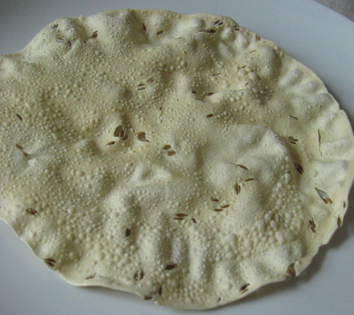
The Appalam or the Pappad as it is called in Northern India is a circular, flattened, wafer thin dry mixture of lentils and spices. It is an almost fat-free, delicious snack if you microwave it although it can also be fried. In particular, the best brand for this test is the Lijjat Pappad. This one is hand made (or used to be). The Lijjat company rose from a tiny all-women cooperative start up in rural India (based on Mahatma Gandhi's principles of self-reliance, theirs is a remarkable and inspiring success story) and is still going strong, producing outstanding Pappads in a variety of flavors.

The idea is pretty simple: The Lijjat Pappad (LP) has a relatively large surface area that covers 75-100% of the circular glass tray in most residential microwaves. Microwave the LP for about 60 seconds and note which of its parts get heated up first (visually seen via a change in color) and how the cooking progresses. Within 60 seconds, you should be able to figure out the hottest and the coldest spots in the oven. In my current residence, the middle of the oven turned out to be the coldest, which was the exact opposite of the result in my prior residence. Of course, this is not intended to be a universal setting and only applies to a subset of foods being heated up.
Why the LP works relatively well for such a test:
1. The consistency of the LP mix is quite remarkable. It is neither thick to resist microwaving, nor too thin and very rarely exhibits any significant warping even after 120 seconds of microwaving (it will simply get carbonized before it warps).
2. The material naturally does not conduct heat well and convection doesn't help much either, so the localized heating effects show up visibly.
3. You can make a meal of your experimental subject once your test is complete. No test goes waste!
No two microwave ovens behave the same way even if they have the same power rating and capacity, and over time they show increased randomness in terms of energy usage and solution quality. Each one has its idiosyncrasies and as you move between apartments over the years, it is irritating to adjusted to a new oven. After you invest all the time in figuring out that the optimal settings to warm your cold coffee is 50 seconds in the previous home, using the same timing with the new one results in a lot of spilled coffee. Furthermore, objects get heated slightly quicker when placed in certain locations of the oven. What is a quick way to optimize your vessel placement and minimize your turn-around time? Enter, the Appalam.
The Appalam or the Pappad as it is called in Northern India is a circular, flattened, wafer thin dry mixture of lentils and spices. It is an almost fat-free, delicious snack if you microwave it although it can also be fried. In particular, the best brand for this test is the Lijjat Pappad. This one is hand made (or used to be). The Lijjat company rose from a tiny all-women cooperative start up in rural India (based on Mahatma Gandhi's principles of self-reliance, theirs is a remarkable and inspiring success story) and is still going strong, producing outstanding Pappads in a variety of flavors.
Why the LP works relatively well for such a test:
1. The consistency of the LP mix is quite remarkable. It is neither thick to resist microwaving, nor too thin and very rarely exhibits any significant warping even after 120 seconds of microwaving (it will simply get carbonized before it warps).
2. The material naturally does not conduct heat well and convection doesn't help much either, so the localized heating effects show up visibly.
3. You can make a meal of your experimental subject once your test is complete. No test goes waste!
Wednesday, May 2, 2012
Optimal Shoelacing
There are gazillion alternative ways to tie your shoelaces of which only a few patterns are easy to remember and possess nice symmetry.

My daughter got her first laced shoes a few weeks ago. As she took it out of the box, the first noticeable thing was that the slack required to tie the laces appeared to be on the shorter side. This posed difficulties for my daughter while she was learning to make those neat knots. Rewiring the shoes resulted in quite a bit of slack, which resulted in big knots that not only helped her learn quickly, but also seemed irresistible to her kindergarten classmates who kept tugging at it. So the aim was to find a lacing pattern that would generate just the right amount of slack.

This is of course an instance of a Traveling Salesman Problem (TSP). Each lace hole represents a city which can be visited exactly once. For example, the slack is maximized by finding the shortest tour, while the slack can be minimized by finding the longest Hamiltonian circuit. Of course, my daughter would prefer finding a good balance between these two extreme solutions, while also ensuring that tightening and loosening the laces are relatively easy to perform. The former objective can be equivalently specified in terms of minimizing deviation from a desired tour length, while the latter requirement can perhaps be approximated by eliminating unfavorable connection patterns and reducing overall friction.

Any OR person will tell you this: just because the TSP is a notorious NP-Hard problem, it does not automatically mean that practical instances are terribly difficult to manage. On the contrary, OR methods excel in quickly finding amazingly (and provably) good answers to practical instances of underlying TSP substructures within decision problems across a variety of industries.

My daughter got her first laced shoes a few weeks ago. As she took it out of the box, the first noticeable thing was that the slack required to tie the laces appeared to be on the shorter side. This posed difficulties for my daughter while she was learning to make those neat knots. Rewiring the shoes resulted in quite a bit of slack, which resulted in big knots that not only helped her learn quickly, but also seemed irresistible to her kindergarten classmates who kept tugging at it. So the aim was to find a lacing pattern that would generate just the right amount of slack.

This is of course an instance of a Traveling Salesman Problem (TSP). Each lace hole represents a city which can be visited exactly once. For example, the slack is maximized by finding the shortest tour, while the slack can be minimized by finding the longest Hamiltonian circuit. Of course, my daughter would prefer finding a good balance between these two extreme solutions, while also ensuring that tightening and loosening the laces are relatively easy to perform. The former objective can be equivalently specified in terms of minimizing deviation from a desired tour length, while the latter requirement can perhaps be approximated by eliminating unfavorable connection patterns and reducing overall friction.

Any OR person will tell you this: just because the TSP is a notorious NP-Hard problem, it does not automatically mean that practical instances are terribly difficult to manage. On the contrary, OR methods excel in quickly finding amazingly (and provably) good answers to practical instances of underlying TSP substructures within decision problems across a variety of industries.
Subscribe to:
Posts (Atom)